Improvements on model

TLDR

As shown in the previous post, the model used to predict the expected goals was promising, but still performed worse than the StatsBomb measure of expected goals. Following some of the suggestions in the previous post, we will show how our model performs as well, if not better, than StatsBomb’s.

What changed from the last results?

We used all the event data available in the database that fulfill two conditions. (1) it’s male football, and (2) the entire competition is available (therefore we didn’t use data where only a subset of games from a competition was available)
We slightly modified the architecture of our model.
We added some features available in the event data regarding the nature of the shot.
We removed some events that were not relevant to our model (e.g. penalties, free-kicks).
We made the validation subset bigger (previously the sizes of subsets were 0.8-0.1-0.1 for training, validation and test sets, now is 0.7-0.2-0.1).

Improvements in the architecture

As mentioned, we are using a Graph Convolutional Neural Network of the subtype message passing. This kind of architecture is fairly small compared to state-of-the-art LLMs, but still contains tens of thousands of parameters. The constraint on the amount of data for training and validation limited severely the amount of layers and the architecture decision in the design of the model. We slightly modified the flow of information inside the model so that the output of the model is calculated from the shooter’s embedding as well as from the goalkeeper’s embedding (previously it was only calculated from the shooter’s embedding).

Adding of “global” features

We called “global” features those that don’t correspond to a single node of the graph but to the graph as a whole. In this case, these features are categorical and attempt to add information about the nature of the play that preceded the shot. These features are:

Play pattern: description of the origin of the play (e.g. regular play, from corner, from throw-in, etc.)
Technique: description of the technique used to make the shot (e.g. normal, volley, diving-header, etc.)
Body part: part of the body used to make the shot (e.g. head, right foot, etc.)
Aerial won (boolean): whether the shot was the product of winning an aerial duel.
Follows dribble (boolean): whether the player performing the shot performed a dribble right before.
First time (boolean): whether the shot is the first touch of the player performing the shot.
Open goal (boolean): whether the shot if performed with an open goal.

Removing events that were not relevant to our model

We noticed that our model had a lot of trouble dealing with some particular shots. Once we analyzed them we noticed that they were penalty and direct free-kicks. For this model we are only interested in open plays, so we decided to remove all the events that were not related to open play.

We might integrate them in the future, but we have a few issues with them in the current implementation:

We don’t have enough data on them to train a model successfully.
The model inputs the global features at the end of the data flow, and it’s processed only by linear layers (and non-linear activation function). Therefore, the expressivity of the model regarding these features is limited, given the complexity of the model itself.

Results

Results on the test subset can be seen in the following scatter plot.

correlation

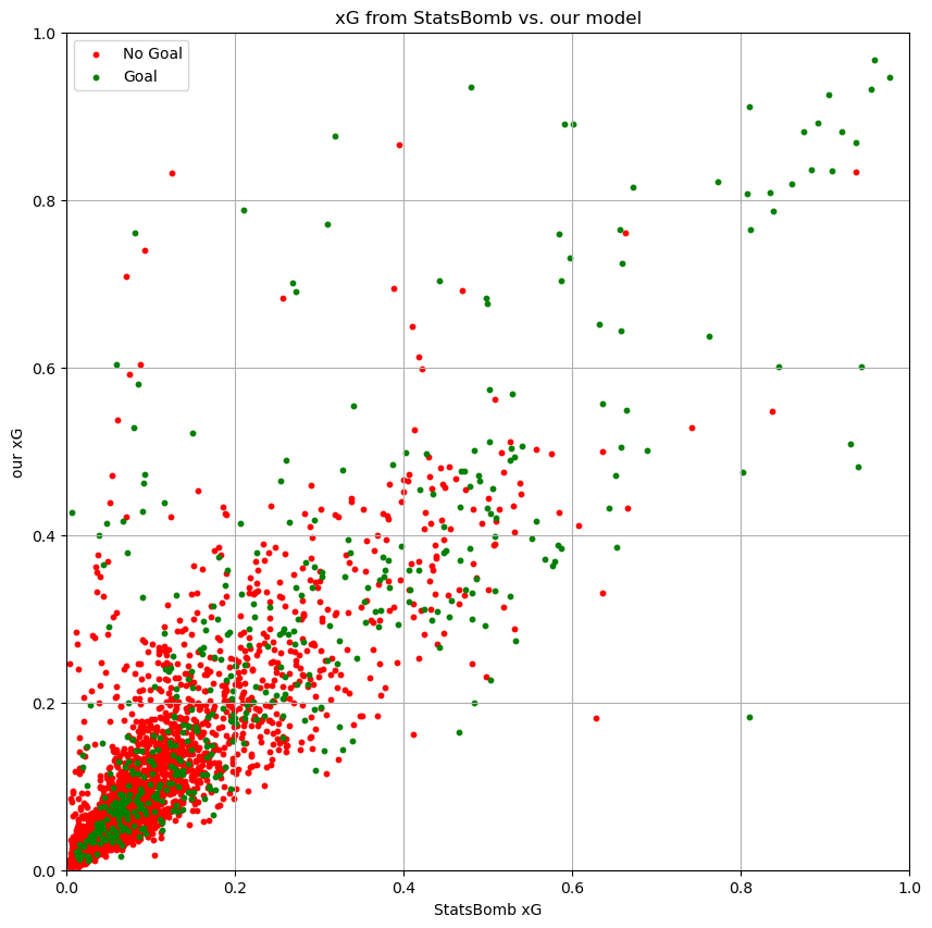
As it can be seen, both metrics are heavily correlated.

sets	Spearman corr	Pearson corr
All shots	0.900	0.858
Just goals	0.818	0.813
Just not goals	0.893	0.837

Comparison with StatsBomb’s xG

We also compared our model’s output with StatsBomb’s xG measure. We used the same data as in the previous post, i.e. the test subset extracted for the whole dataset.

As in the previous post, we use Brier score and AUC to compare the two metrics. Here we also introduce the Crossentropy between both approximations of xG and the empirical distribution of goals (Wikipedia page).

model	Brier score	Crossentropy	AUC
StatsBomb xG	0.0730	0.2561	0.8128
our XG	0.0727	0.2535	0.8207

These results do not allow to state that one model is better than the other, but they do show that our model is not worse than StatsBomb’s xG. We will explore the differences:

Distribution of data

distribution_all

distribution_goals

distribution_non_goals

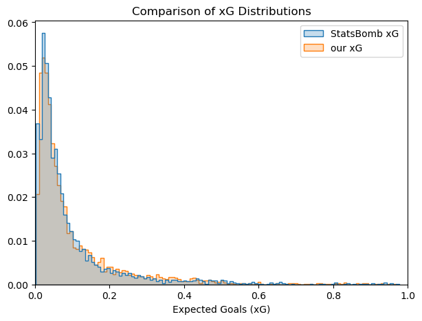
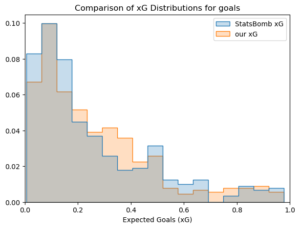
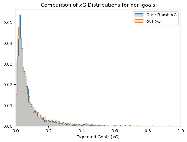
The comparison of the distribution of the predictions from the two models shows some interesting trends:

Distributions look very similar.
Small differences can be appreciated, with StatsBomb xG score more commonly values between 0 and 0.15 and our model scores more commonly between 0.2 and 0.4.

Angle variation evaluation

We intend to measure the effect that the angle of the shot has on the xG. For this, we obtained the xG from shots with only the shooter and the goalkeeper. The keeper is in the middle of the goal and the shot is performed 11 meters away from the goalkeeper. 20 shots are performed in angles from 100° to 260° (from 10° to 170° if considered from the end line), as shown in the following images:

angle_100 Shot performed from 100°

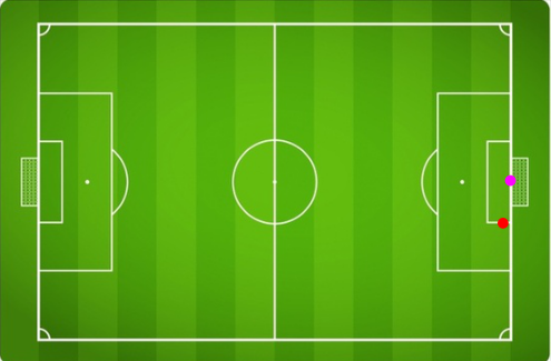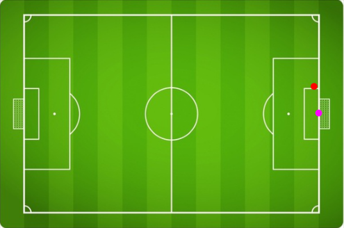angle_260 Shot performed from 260°

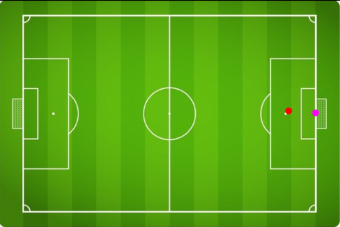angle_184 Shot performed from 184°

The xG from this positions with different body parts hitting the ball can be seen in the following figure: xg_vs_angle

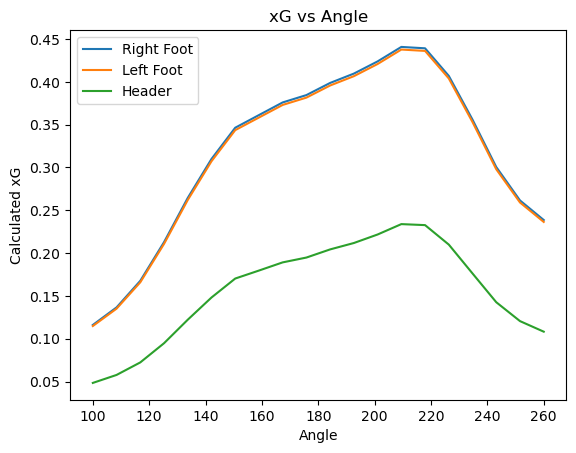
Some interesting things that can be extracted from this:

The xG is not symmetric concerning 180°, meaning that, according to the model, it is more probable to score from the right side of the field (from the goalkeeper’s point of view) than from the left side: - The model is trained with the data without any constraint concerning the side where the shot is performed, hence we can assume that this is, approximately, the distribution of goals from each angle. The reason for the asymmetry is probably due to the majority of players being right-footed, therefore having more chance to score from the right side. - The asymmetry may not be a desirable feature, since the model might be intended to be as naive as possible. This can be fixed by reflecting all the positions of the players with respect to a line that goes through 180° (a line from goal to goal) in a way that the shots are always performed from one side of the field.
There is no major difference in the shape of plots for the different body parts considered, just in the magnitude. This is particularly the case when comparing right and left feet, where the differences are very small. One might expect shots from the left side of the field to be more precise with the left foot, which is not the case. This can have two explanations for this: - Architectural reason: As mentioned before, global features, such as the body part, are integrated into the data flow at a later stage, and are only processed by linear layers and non-linear activations layers, limiting the ability of the model to capture this phenomena. - Statistical reason: Since the model does not have information about the player performing the shot, it does not also have information on the dominant foot of the player. Therefore, since most players are right-footed, it’s possible that many shots taken from the left side with a left foot are performed by a right-footed player.
The shape of the plots seems to be smooth, which is a nice property in this kind of function.

Examples

Let’s considerer some cases from top left corner of scatter plot, meaning, shots where our model score high and StatsBomb model score low:

Goals:

Lyon - Monaco 2015-16
StatsBomb xG: 0.60025674
our xG: 0.89113533
link
Fifth goal, second half from corner
Keeper not in goal, just a defender

goal_lyon

Lazio - Udinese 2015-16
StatsBomb xG: 0.3183885
our xG: 0.8764055
link
First goal
Tap in from a cutback

goal_lazio

Crystal Palace - Chelsea 2015-16
StatsBomb xG: 0.59007293
our xG: 0.8907189
link
Third goal by Diego Costa
No keeper on goal, just a defender

goal_chelsea

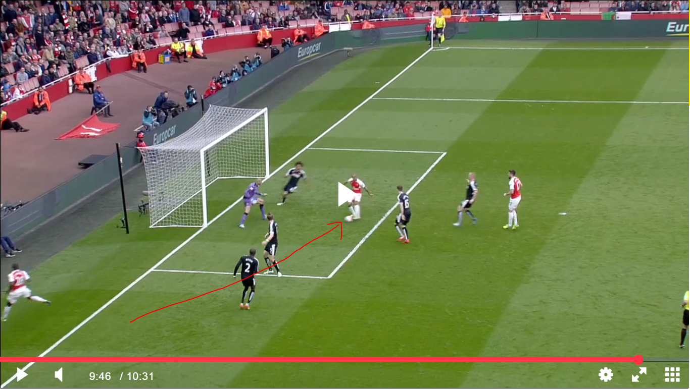
Arsenal - Watforf 2015/16
StatsBomb xG: 0.47959393
our xG: 0.9349653
link
Last goal by walcott
Tap in from cutback

goal_arsenal

Not goals:

Atalanta - Roma 2015/16
StatsBomb xG: 0.3948238
our xG: 0.8656543
(couldn’t find video from it)
Džeko shot at minute 81

Crystal Palace - Aston Villa 2015/16
StatsBomb xG: 0.12405383
our xG: 0.86449665
(couldn’t find video from it)
Bakary Sako shot, minute 47

Let’s now consider cases from the bottom right corner, i.e., shots where our model scored low and StatsBomb scored high:

Goals:

Athletic - Bilbao 2015-16
StatsBomb xG: 0.8093721
our xG: 0.1830449
link
Third goal from Athletic (3-0)
shooter completely alone after offside line push from defense

goal_athletic

Manchester City - Stoke City 2015-16
StatsBomb xG: 0.92961997
our xG: 0.5092157
link
last goal (4-0)
forward evades keeper

goal_mancity

Manchester City - Norwich 2015-16
StatsBomb xG: 0.93852484
our xG: 0.48162717
link
norwich goal (1-1)
keeper losses the ball

goal_norwich

Carpi - Bologna 2015-16
StatsBomb xG: 0.8017068
our xG: 0.47479144
link
bologna first goal (1-1)
captures rebound from the post\

goal_bologna

Discussion

Regarding the top left cases, at least the cases that ended in goals, there seem to follow a clear pattern, where our model scores very high on two play patterns, 1) where the keeper is not in position to protect the goal, but there is a defender that is, and 2) in short range tap-ins from cutbacks.

The first case makes sense given that our architecture extracts most of the data to predict a goal or not from the graph embeddings of the shooter and the goalkeeper. If the goalkeeper is not covering the goal, it might generate a big effect. The second case is extremely interesting since among the inputs there is no information regarding the kind of pass that preceded the goal, hence the model is making the decision based only on the positions of the keeper and defenders. A particularity of cutbacks, and why they are so dangerous, is that they generate situations in which the goalkeeper needs to remain close to the goal, ensuring that the eventual shot is very close to the goal but not to the goalkeeper.

With respect to the bottom right cases. They all seem to be instances that occur rarely and it could be expected that the training set did not contain enough cases to calibrate the model properly. This is an inherent characteristic of deep learning models and can be addressed by removing rare cases (for instance, by removing categories of a feature with few occurrences, combining them with others), or by increasing the dataset.

Future work

The database used consider only men games. According to an analysis performed by StatsBomb, data from both gender can be used to train one model and include the gender as a feature. This is a quick way to increase the dataset.
The implementation evaluated here is optimized for xG and would need slight modifications (mainly on the last layers) to be used as tactical advantage scoring system, which is the long term goal of this project.
A model for direct free kicks could be trained, although probably the current models work as good as possible in that particular department.
Information about the previous events could be added. In fact, shot events in StatsBomb database have a list of related events as well as a reference to the event capturing the key pass that allows the shot, if there is one.